3D Brain Tumour Segmentation
Five deep learning architectures trained on 3D brain MRI scans, from a CNN baseline to a Transformer. A 2.4M-parameter model matched a 62M-parameter one. Everything built and benchmarked from scratch on a consumer GPU.
TL;DR
I trained and compared five 3D segmentation architectures on the BraTS2021 brain MRI dataset, starting from a CNN baseline and progressing through gated attention, a global Transformer, a 3D adaptation of a 2026 KAN hybrid paper (extended from 2D to volumetric inference), and a controlled KAN ablation. Every model was trained on a GTX 1070 Ti (8 GB VRAM) using only 150 of the available 1,251 training cases, a hardware constraint that turned out to produce some genuinely interesting results. I went in expecting the Transformer to dominate and left with a very different picture.
The headline finding: A 22M-parameter CNN with attention gates outperformed a 62M-parameter Transformer. A 2.4M-parameter KAN hybrid then matched the Transformer at 26× fewer parameters. And a controlled ablation (one variable changed, everything else identical) showed that swapping just the bottleneck activations for KAN splines narrowly beat the attention mechanism on the most clinically important metric, all while using 12% of the available data.
The Problem
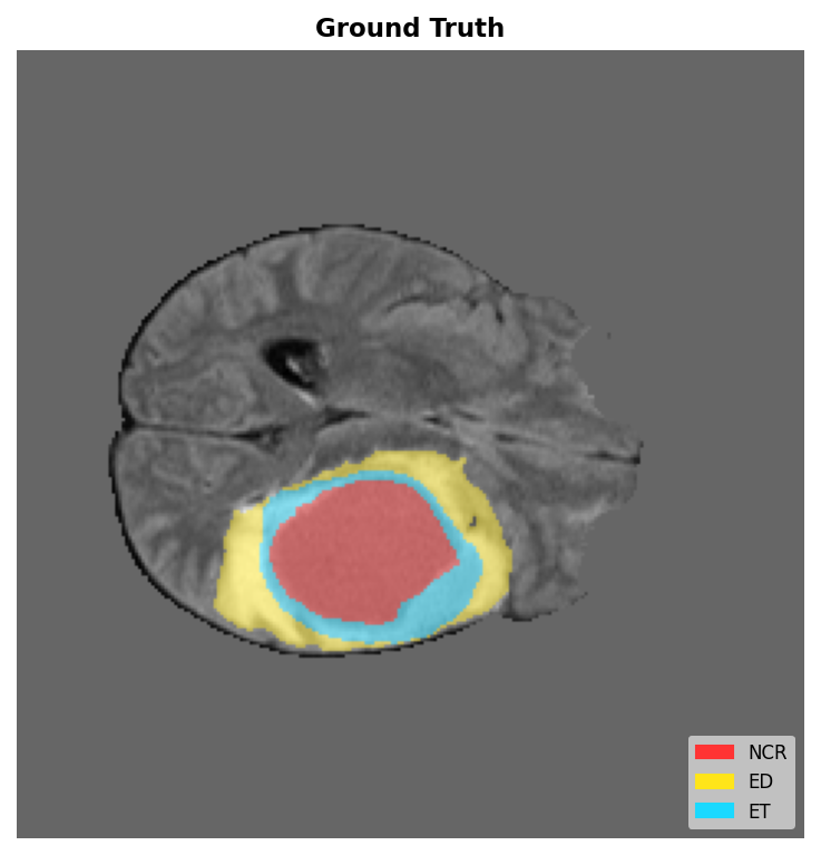
Brain tumours don’t behave predictably. They’re irregular in shape, vary enormously between patients and are comprised of different tissue sub-types including a necrotic core (NCR), a surrounding ring of oedema (ED) and a patch of actively growing enhancing tumour (ET). These tissue types all look different depending on which MRI sequence you’re looking at. Radiologists usually delineate them by hand in a process that’s slow and prone to include a bias that varies between clinicians.
Automating 3D segmentation is interesting because it feeds directly into clinical decisions: surgery planning, radiation targeting, and tracking whether a treatment is actually shrinking the tumour. Getting it right, and knowing where the model is uncertain are two very important aspects.
The challenge dataset defines three clinically meaningful sub-regions, each evaluated separately because they’re used for different purposes:
| Region | Composed of | Clinical use |
|---|---|---|
| WT - Whole Tumour | NCR + ED + ET | Surgery planning (how much tissue is affected) |
| TC - Tumour Core | NCR + ET | Core characterisation (the actively dangerous region) |
| ET - Enhancing Tumour | ET only | Treatment response (is the tumour actually shrinking?) |
The Dice coefficient
The primary metric is the Dice coefficient, which measures how well the model’s prediction overlaps with the ground truth label drawn by an expert radiologist. It ranges from 0 (no overlap whatsoever) to 1 (perfect agreement).
If you think of two sets of highlighted voxels on a brain scan, a set of voxels the model predicts as tumour P, and a set the radiologist actually labelled as tumour G. The Dice coef. would give us the fraction of voxels that both P and G classify as a tumour, to be more precise:
| Term | Meaning |
|---|---|
| |P ∩ G| | Voxels where both the model and the expert said "tumour" (the overlap) |
| |P| | How many voxels the model predicted as tumour |
| |G| | How many voxels the expert labelled as tumour |
| Factor of 2 | Ensures a perfect prediction (P = G) scores 1 rather than 0.5 |
If the model predicts perfectly, \(P = G\), the overlap equals both sets, and Dice = 1. If the model misses everything, the overlap is zero and Dice = 0. A model that marks too much as tumour gets penalised too: a large \(\lvert P \rvert\) inflates the denominator without helping the numerator.
A score of 0.88, roughly what this project achieves, means the model’s tumour outline agrees with the expert label about 88% of the time. As you’ll see below, that puts it in competitive territory with models trained on the full 1,251-case dataset.
Dataset & Hardware Reality
The Brain Tumour Segmentation 2021 Challenge dataset has 1,251 pre-operative multi-parametric MRI scans, each with four aligned modalities and an expert-drawn voxel-level mask.
| Cases | 1,251 patients |
| Modalities | FLAIR - T1 - T1CE - T2 (4 channels) |
| Volume shape | 240 × 240 × 155 voxels, 1 mm isotropic |
| Labels | 0 (background) - 1 (NCR) - 2 (ED) - 4 (ET) |
| Colour scheme | NCR = red - ED = yellow - ET = cyan |
Why only 150 cases?
The honest answer is hardware. This project ran on a GTX 1070 Ti, a consumer GPU with 8 GB of VRAM and no Tensorcores. That’s a real constraint when dealing with 3D medical volumes.
A single brain scan is 240×240×155 voxels across four modalities. Loading one full volume into GPU memory takes several gigabytes on its own; there’s simply no way to run a full forward-backward pass on a complete brain at once. The workaround is patch-based training: randomly crop 128×128×128 sub-volumes and train on those instead, using MONAI’s foreground-biased sampler to ensure the model sees tumour-containing patches more often than pure background.
Even with patches, training one model on all 1,251 cases would take several days of wall-clock time. With four architectures to compare, that’s weeks, which isn’t a realistic timeline for a personal project. Capping at 150 training cases and 50 validation cases keeps each run to a manageable window while still being large enough to tell whether an architectural change is genuinely helping.
The same fixed split, generated once with a random seed and reused for every model, ensures the comparisons are fair. Any Dice difference is an architecture signal, not a data split artefact.
The practical rhythm was overnight training sessions: kick off a run before bed, check the numbers in the morning. The CNN models landed at roughly 7 hours each; Swin UNETR took 17. At one point I looked into renting cloud compute. For roughly the cost of a coffee you could run Swin UNETR on the full 1,251 cases on a V100 in a few hours. I decided against it. The point of the project was understanding the architectures and building the pipeline, not chasing the best possible number. That said, it’s an easy upgrade path if I ever come back to it.
What genuinely surprised me was how competitive the numbers ended up being. The Attention U-Net’s TC score of 0.884 came within 0.004 of the BraTS2021 challenge winner, which trained on the full 1,251 cases with serious compute. The ET score outright beats both the original Attention U-Net paper’s published range and Swin UNETR’s full-dataset results. I didn’t expect that going in, and the pattern held across every model I trained. For this problem, at least in this data regime, architectural choices seem to matter as much as data volume.
Segmentation Overlays
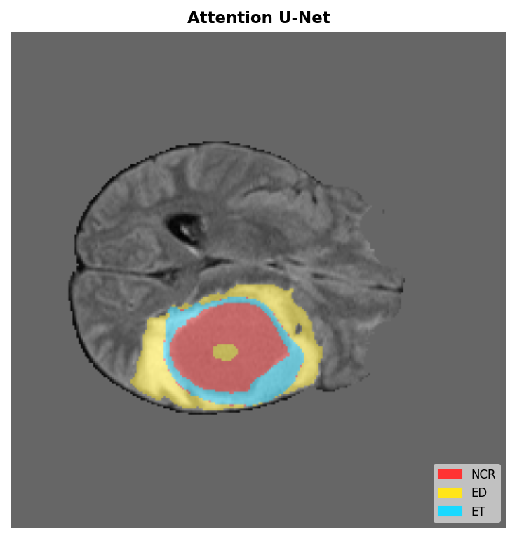
Drag the handle to compare Ground Truth (left) against the Attention U-Net prediction (right) on case BraTS2021_01619, axial slice 67 (a validation case with strong representation of all three tumour regions).
Architecture Exploration
Rather than picking a single architecture and optimising it, I designed this as a progression. Each model was chosen to answer a specific question raised by the previous one’s results. The story goes from local to global, and then back again.
The skip connections carry all encoder features directly into the decoder, including background regions that have nothing to do with the tumour. The model has no way to filter that out, which pushes it toward over-predicting.
The attention gates help the model focus on tumour-relevant regions in the skip connections. But each convolution still only looks at a small patch of nearby voxels at a time, so the model cannot reason about the tumour shape or context across the full brain.
The Transformer has 62 million parameters but only 150 training cases to learn from. With that ratio it ends up memorising training patches rather than generalising, and scores worse than the much smaller CNN.
This model changes several things at once compared to the baseline: fewer convolutions per level, a lighter bottleneck, and KAN activations. If it performs differently there is no clean way to know which change is responsible.
3D U-Net (Model 1, CNN Baseline)
Çiçek et al. 2016 — “3D U-Net: Learning Dense Volumetric Segmentation from Sparse Annotation”
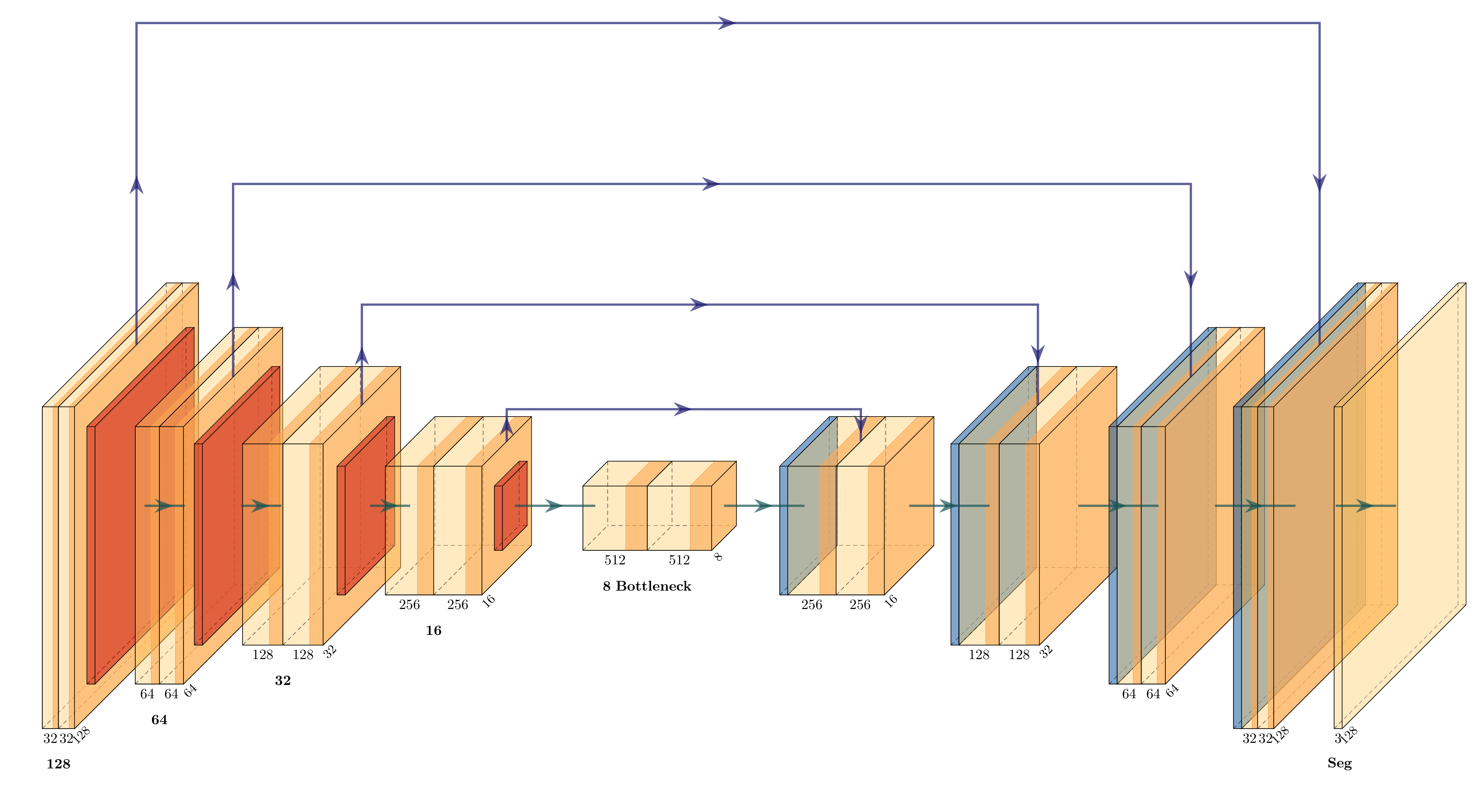
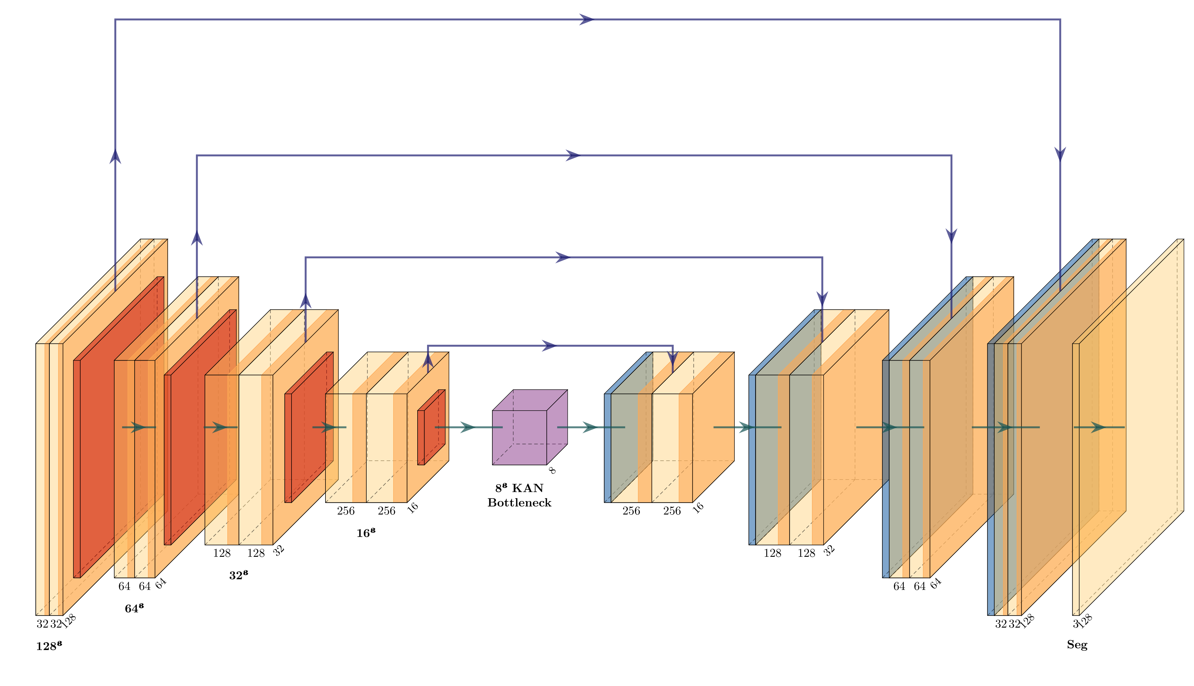
The starting point for almost any 3D medical segmentation task. An encoder compresses the volume down through four spatial levels (halving resolution each time via max-pooling), a bottleneck processes the most abstract features, and a decoder mirrors the encoder back up, with skip connections carrying fine-grained spatial detail from each encoder level to the corresponding decoder level.
Building this first was important for a reason beyond the Dice score. It establishes the full training pipeline that every later model inherits unchanged. The patch sampler, the sliding-window inference, the BraTS metrics, the MLflow logging. All comparisons are relative to this foundation.
Where it falls short: A 3×3×3 convolution kernel sees 27 neighbouring voxels at a time. That’s fine for local texture and edges, but brain tumours have long-range spatial structure. The shape of the enhancing tumour rim on one side relates to the necrotic core on the other. Without many stacked layers, the model can’t reason across that distance. And the skip connections pass everything from encoder to decoder, including background activations that push the decoder toward over-segmenting.
| Region | WT | TC | ET | Mean | Train time |
|---|---|---|---|---|---|
| Dice | 0.876 | 0.877 | 0.869 | 0.874 | ~7 hrs |
Attention U-Net (Model 2)
Oktay et al. 2018 — “Attention U-Net: Learning Where to Look for the Pancreas”
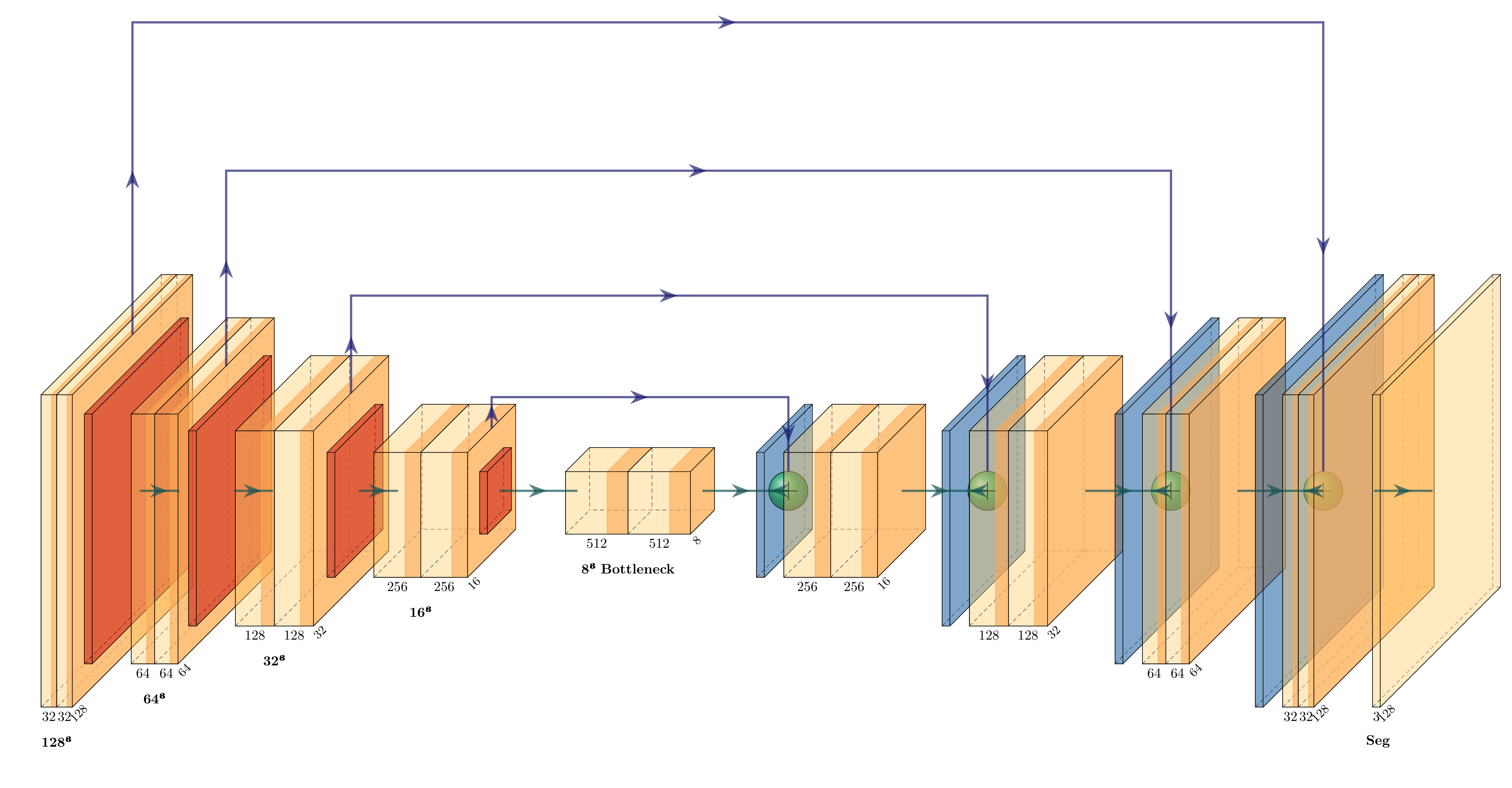
Before abandoning convolutions entirely, can we make the skip connections smarter? The Attention U-Net keeps the same encoder-decoder structure but adds a gating mechanism to each skip connection. Before encoder features get concatenated into the decoder, they pass through an attention gate that learns a spatial soft-mask, amplifying activations in tumour-like regions and suppressing them in background.
The gate is learned entirely from the segmentation loss with no extra supervision. The decoder generates a gating signal at each resolution level and compares it to the encoder’s features. Where they agree (this looks like tumour), the gate opens. Where they don’t, it closes.
\[\alpha = \sigma\!\left(W_\psi \cdot \text{ReLU}(W_g \cdot g + W_x \cdot x + b_g)\right)\]This is the mechanism visualised in the attention heatmaps further down the page.
ET was the region I expected to benefit most. It’s compact, has irregular boundaries, and is hardest to distinguish from surrounding tissue. The results confirmed what I expected.
| Region | WT | TC | ET | Mean | Params | Train time |
|---|---|---|---|---|---|---|
| Dice | 0.886 | 0.884 | 0.875 | 0.882 | 22.66M | ~7 hrs |
How this compares to published results (all trained on the full 1,251 cases):
| WT | TC | ET | |
|---|---|---|---|
| 150 case Attention U-Net | 0.886 | 0.884 | 0.875 |
| Published Attention U-Net (Oktay 2018) | 0.88–0.90 | 0.82–0.87 | 0.78–0.83 |
| BraTS2021 challenge winner (nnU-Net) | 0.932 | 0.888 | 0.884 |
TC and ET both beat the original paper’s published range, on 12% of the data. TC is within 0.004 of the BraTS2021 challenge winner.
Swin UNETR (Model 3)
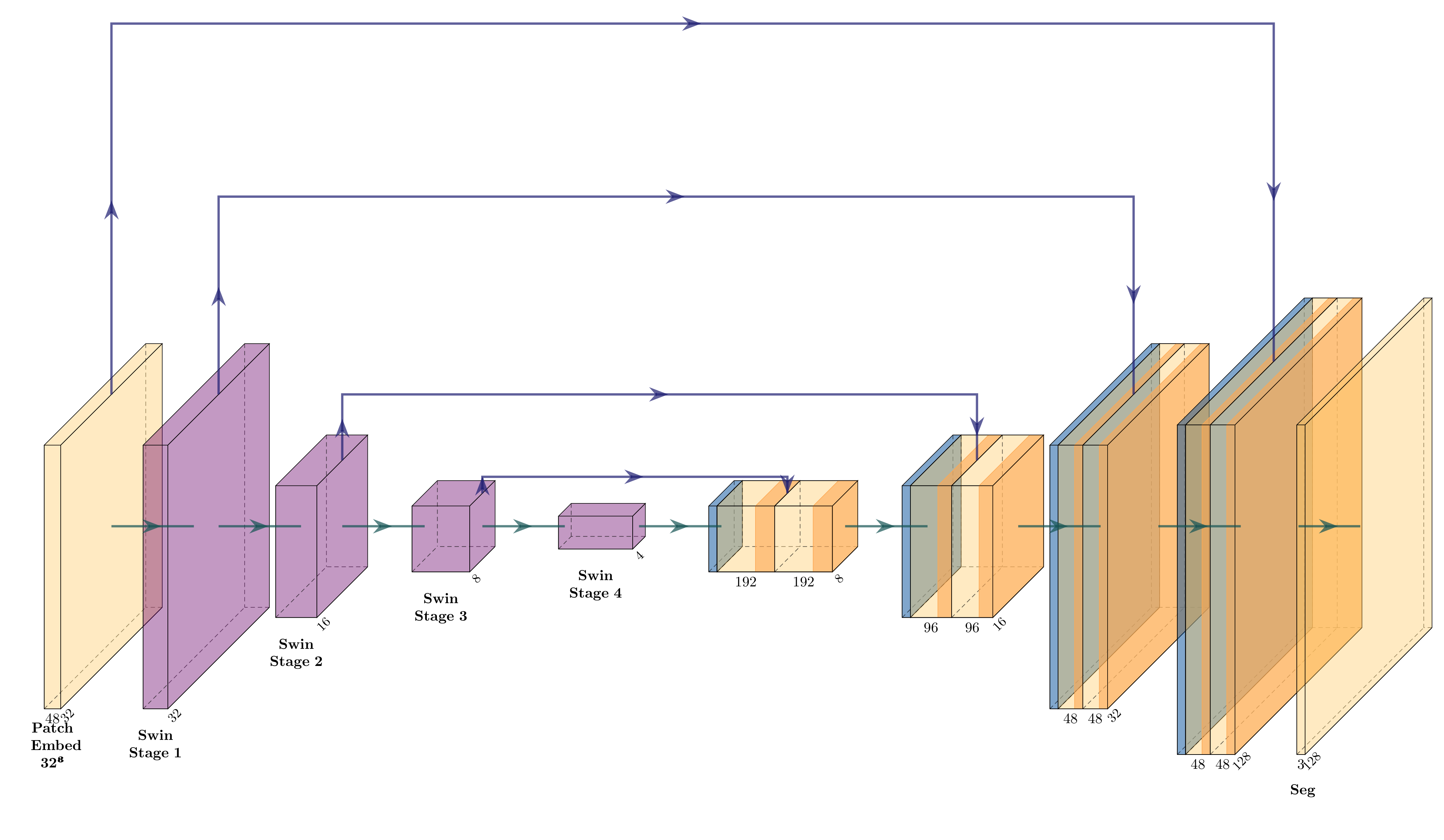
Hatamizadeh et al. 2022 — “Swin UNETR: Swin Transformers for Semantic Segmentation of Brain Tumors in MRI Images”
Attention gates help, but they still operate on convolutional features. The locality constraint is baked into the convolution itself, not just the skip connections. The natural next question is what happens if we replace convolutions with a mechanism that has no locality constraint at all.
Swin UNETR does exactly that. It tokenises the 3D volume into small patches and passes them through a hierarchical Swin Transformer encoder, where every token attends to every other token within its local window and those windows shift between layers to allow global context to accumulate. A voxel near the front of the brain can, in principle, directly influence predictions near the back. The decoder stays CNN-based, keeping the upsampling path efficient.
| Region | WT | TC | ET | Mean | Params | Train time |
|---|---|---|---|---|---|---|
| Dice | 0.882 | 0.863 | 0.862 | 0.869 | 62.19M | ~17 hrs |
Swin UNETR lost to the Attention U-Net (0.869 vs 0.882 mean Dice) despite having 2.7× more parameters and taking roughly 17 hours to train.
This was the result I found most interesting, and honestly the one I hadn’t predicted going in. I expected the Transformer to at least match the CNN at full-volume evaluation, given that it clearly did better at the patch level (0.855 vs 0.834). It didn’t. Looking back, three things were compounding each other. Sixty-two million parameters on 150 cases is a bad mismatch from the start (the gap between patch-level validation and full-volume evaluation is the textbook sign of memorising patch patterns rather than generalising). And the patch training specifically undermined the thing that was supposed to make Swin UNETR worth the extra cost. It was trained on 128³ crops and never once saw a complete brain, so the attention mechanism designed for global context never actually got global context to work with. On top of that, CNNs have a built-in spatial locality prior that turns out to be a useful assumption for medical images, and it generalises well from limited examples in a way that Transformers, which learn spatial structure from scratch, simply don’t.
More parameters and global attention don’t automatically mean better results. With limited data, a well-designed CNN with targeted attention outperforms a 4× larger Transformer.
KAN U-Net (Model 4, 3D U-KABS)
Liu et al. 2024 — “KAN: Kolmogorov-Arnold Networks” (ICLR 2025)
arXiv:2602.07702 — “A hybrid Kolmogorov-Arnold network for medical image segmentation”
Swin UNETR’s result reframes the whole question. If a bigger, more powerful model failed because it had too many parameters for the available data, what happens if we go in the opposite direction? How small can we make the model before performance collapses?
Originally, the plan was to implement CDA-Mamba here (a recent state-space model that seemed like a natural successor to Swin UNETR, replacing the Transformer’s quadratic attention cost with linear state-space scanning). I hit a wall. mamba-ssm has no official Windows wheels, and getting it to compile from source against the right CUDA version was not a quick afternoon. Rather than spend days fighting the environment, I switched to KAN U-Net, a 2026 paper, also recent, also non-standard, and pure PyTorch with no exotic dependencies. In hindsight that pivot worked out well, because the KAN result turned out to be the most interesting one in the whole project.
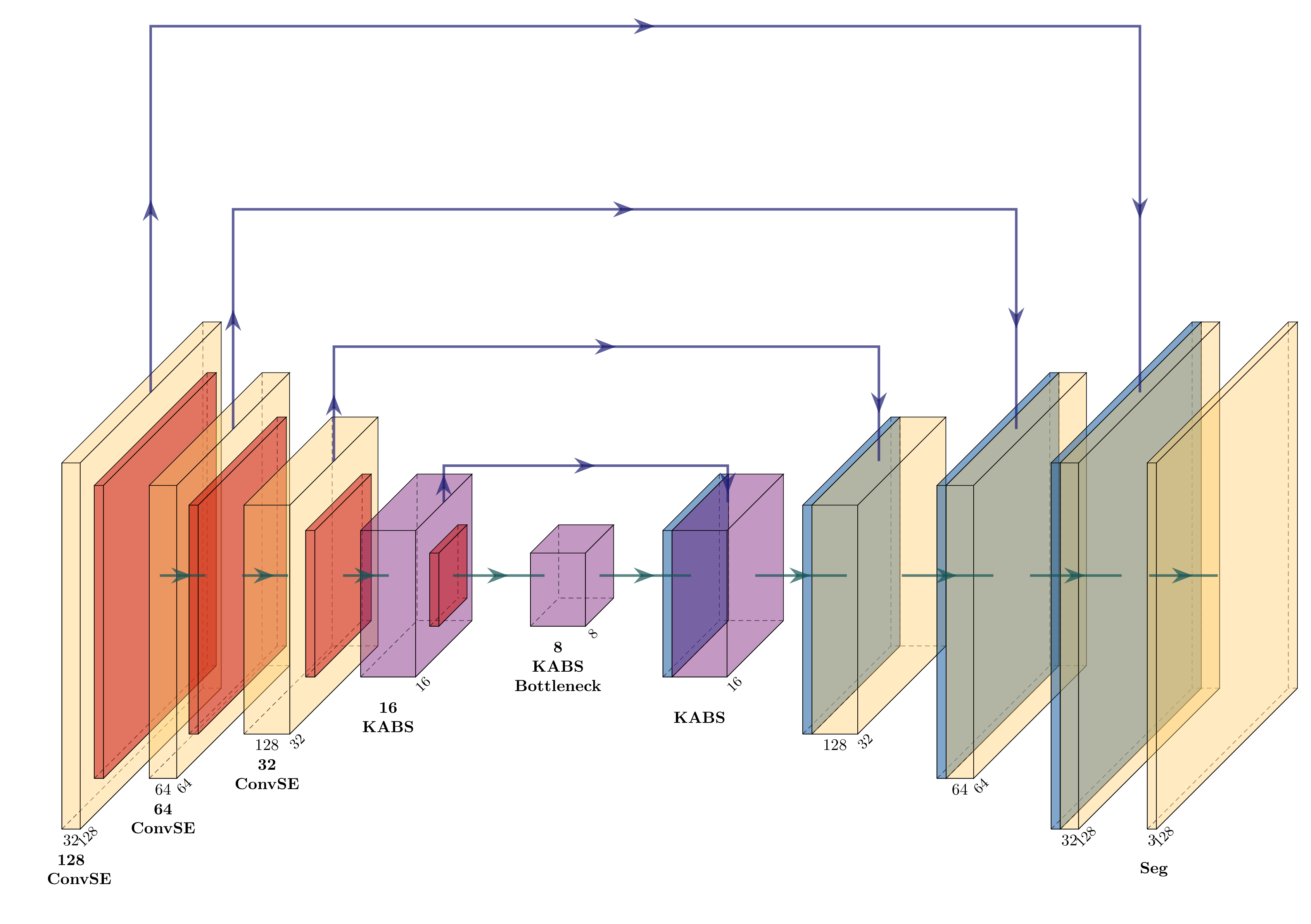
KAN U-Net is the experiment that tests the lightweight direction. It’s a 3D U-Net backbone where the standard activations at the two deepest spatial levels are replaced with KAN (Kolmogorov-Arnold Network) activations, learnable spline functions rather than fixed nonlinearities. The rest of the architecture stays slim, with a single convolution per level, a depth-wise separable bottleneck, and squeeze-and-excitation channel attention. Total parameter count is 2.42M.
The key idea behind KANs is that in a standard network, the weights are learnable but the activation functions (ReLU, GELU) are fixed shapes. KANs flip this: the activations themselves become learnable curves that adapt during training. The theoretical basis is the Kolmogorov-Arnold representation theorem, which states that any continuous function can be broken down into compositions of simpler single-variable functions.
Two curve types are used per block. One uses smooth global curves suited for capturing the broad shape of the tumour, called KAB (Bernstein polynomials). The other uses locally adaptive curves better suited for fine-grained boundary detail, called KAS (B-splines).
| Region | WT | TC | ET | Mean | Params | Train time |
|---|---|---|---|---|---|---|
| Dice | 0.878 | 0.873 | 0.856 | 0.869 | 2.42M | ~7 hrs |
KAN U-Net ties Swin UNETR’s mean Dice (0.869) at 26× fewer parameters. The Transformer needed 62 million parameters and 17 hours of training; this got there with 2.42 million in a fraction of the time.
KAN 3D U-Net (Model 5, Ablation)
Something that had been nagging at me was that the U-KABS architecture (KAN U-Net) differs from the 3D U-Net in more than just its activations. It also uses single convolutions per level, a depth-wise bottleneck, and SE channel attention. So even if U-KABS performs well, you can’t cleanly attribute that to the KAN activations specifically. To settle the question, I ran a controlled ablation using the exact same 3D U-Net architecture, with the single change of replacing the two LeakyReLU activations in the bottleneck with KAN activations (Bernstein + B-spline). Every encoder block, every decoder block, every skip connection, unchanged. Only the bottleneck activation function differs.
That gives a clean ablation, one variable changed and everything else kept identical.
| Region | WT | TC | ET | Mean | Params | Train time |
|---|---|---|---|---|---|---|
| Dice | 0.879 | 0.885 | 0.869 | 0.878 | 22.59M | ~7 hrs |
The TC score of 0.885 narrowly beats the Attention U-Net (0.884), the model specifically designed to improve TC through learned gating. I’d need multiple seeds to be sure the 0.004 mean improvement is a real signal rather than noise, but the direction is consistent. What’s clear is that KAN activations at the bottleneck don’t hurt, and might give a modest benefit at the most semantically complex layer of the network.
Results Summary
Sorted by mean Dice (descending). All models: GTX 1070 Ti, 150/1,251 training cases, identical pipeline.
| Model | WT | TC | ET | Mean | Params | Train time | Notes |
|---|---|---|---|---|---|---|---|
| Attention U-Net | 0.886 | 0.884 | 0.875 | 0.882 | 22.66M | ~7 hrs | Best overall; TC and ET beat published full-data results |
| KAN 3D U-Net | 0.879 | 0.885 | 0.869 | 0.878 | 22.59M | ~7 hrs | Ablation: KAN bottleneck only; TC beats Attention U-Net |
| 3D U-Net | 0.876 | 0.877 | 0.869 | 0.874 | 22.58M | ~7 hrs | Baseline |
| Swin UNETR | 0.882 | 0.863 | 0.862 | 0.869 | 62.19M | ~17 hrs | Beaten by CNN despite 2.7× more params |
| KAN U-Net | 0.878 | 0.873 | 0.856 | 0.869 | 2.42M | ~7 hrs | Ties Transformer at 26× fewer params |
All models trained on the same 150 of 1,251 cases, on a GTX 1070 Ti, using identical training pipelines. The comparisons between architectures are what matter here. Absolute scores are below full-dataset published results, but that’s a data volume issue, not an architecture one.
Compare Any Two Models
Pick which predictions to put on each side of the divider, then drag the line to reveal one under the other.
Drag the divider to reveal one prediction under the other. Case BraTS2021_01619, axial slice 67.
3D Tumour Mesh
The segmentation mask isn’t just a 2D outline. It’s a full 3D volume. Running Marching Cubes on the ground truth label converts each sub-region into a triangulated surface mesh. The translucent grey shell is the brain surface itself, extracted from the skull-stripped FLAIR image, giving a sense of where the tumour sits anatomically and how large it is relative to the surrounding tissue.
Drag to rotate, scroll to zoom. Click legend entries to toggle regions on and off.
Case BraTS2021_01619 ground truth, rendered with Marching Cubes. Brain surface (step size 5, 7k verts) · NCR red (3.9k verts) · ED yellow (10.2k verts) · ET cyan (7.8k verts).
Attention Gate Heatmaps
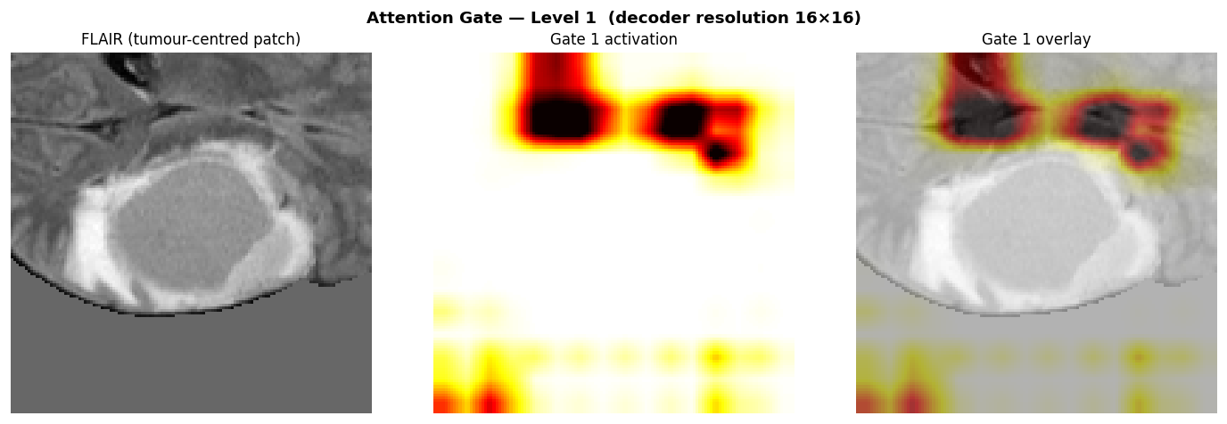
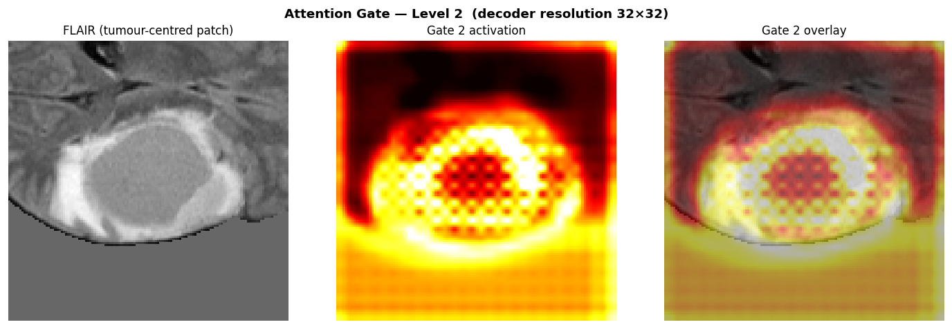
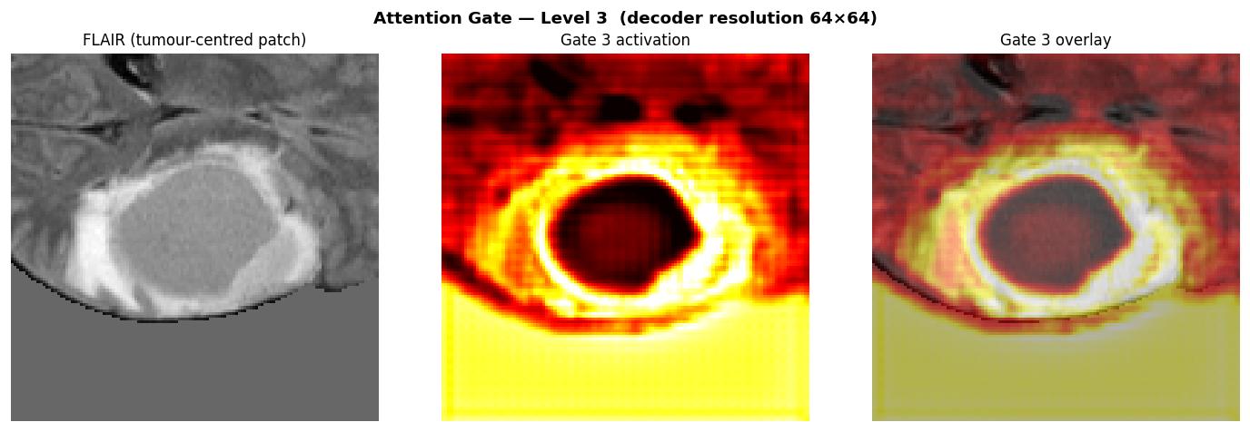
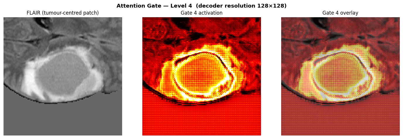
One of the nicer things about the Attention U-Net is that it produces interpretable outputs beyond the segmentation mask. The attention gates generate a spatial weight map at each decoder level. Values close to 1 mean the gate is open (these encoder features get passed through); values close to 0 mean they’re suppressed. Bright regions are where the model is focusing.
These were extracted by registering forward hooks on each AttentionGate3d module during a single forward pass on a tumour-centred 128³ patch. Each image shows three panels: the raw FLAIR crop (left), the gate activation heatmap (centre), and the gate overlaid on FLAIR (right). All three panels are spatially aligned to the same patch.
Uncertainty Heatmap (Test-Time Augmentation)
Knowing where the model is confident matters as much as the prediction itself. The maps below were produced using the Attention U-Net, the best-performing model in this comparison. To get a per-voxel confidence estimate without any architectural changes, I ran inference 8 times, each time with a different combination of axis flips applied to the input and then undone on the output. Averaging these 8 predictions gives a more robust final mask, the per-voxel standard deviation across them gives an uncertainty map.
The intuition: if the model gives the same answer regardless of how the brain is oriented, it’s confident. If the answer shifts with orientation, something there is ambiguous.
High uncertainty (bright yellow-red) clusters at tumour boundaries, which is exactly where a radiologist would want to double-check. The NCR/ED transition, where necrotic core meets the surrounding oedema, is consistently the most uncertain region across patients.

Interactive Charts
Model Comparison
Radar Chart
Parameter Efficiency
Training Curves
The val Dice lines jump around quite a bit, and that’s worth explaining. Each validation pass during training runs on random 128³ patches (not the full brain). With only 50 val cases in the pool, any given epoch might happen to sample more background-heavy regions, or catch the enhancing tumour edge on every case, and that swings the aggregate Dice by a few points in either direction. It’s sampling noise, not instability. The final numbers in the results tables are a different story. Those come from sliding-window inference across the entire volume, which averages all of that out and is why the reported scores are both more stable and a bit higher than the mid-training curves suggest.
Architecture Diagrams
Engineering Decisions
A few decisions that shaped how the project ran. Some were kind of obvious, and some less so.
npy preprocessing cache
NIfTI loading via nibabel is roughly 100× slower than loading a numpy array. Since every training run iterates over 150 cases per epoch for 100 epochs, that overhead adds up fast. Running a one-time preprocessing pass to convert everything to float16 .npy files brings per-epoch data loading from minutes to milliseconds. It's the kind of thing that seems like an optimisation detail but actually changes what's practical to experiment with.
Patch 128³, batch size 1, fp16
A full BraTS volume (240×240×155 across 4 modalities) doesn't come close to fitting in 8 GB of VRAM. The workaround is random 128³ crops with foreground-biased sampling, so the model sees tumour tissue more often than background. Batch size 1 and fp16 mixed precision (torch.cuda.amp) are both required to stay within VRAM. The GradScaler handles fp16 gradient underflow automatically.
BCEDiceLoss (50/50 blend)
Dice loss alone is unstable early in training. When all predictions are near-zero at initialisation the gradient nearly vanishes. Blending in equal parts BCE provides a stable signal from epoch 1. The 50/50 ratio is a standard BraTS starting point and I didn't find a reason to change it.
AdamW (lr 1e-4, weight decay 1e-5)
In standard Adam, weight decay is folded into the gradient update, which means the effective regularisation varies across parameters depending on their gradient magnitude. AdamW decouples the two, penalising every parameter proportionally to its own magnitude and independently of the gradient. In practice this generalises better, especially for large models like Swin UNETR. The same lr and weight decay are shared across all five models with no per-architecture tuning.
Fixed train/val split (seed 42)
All five models train and evaluate on the exact same 150/50 case split, generated once and saved to splits.json. Without this, a single fortunate or unfortunate random draw could explain a 0.003 Dice difference between two models. With a fixed split, any difference is the architecture, not the data lottery.
MLflow (local SQLite)
All hyperparameters and per-epoch metrics logged automatically to a local SQLite database. No server required. The training curves chart on this page pulls directly from that database. The graphs are a literal record of what happened during training, not reconstructed after the fact.
KAN activations in fp32
Bernstein polynomial evaluation involves computing x⁴, which loses enough precision in fp16 to destabilise training. The KAN forward pass casts to fp32 internally regardless of the surrounding AMP context. Small detail, took a while to find.
What’s Next
Training on the full dataset is the most direct continuation. WT is the most volume-sensitive region, spatially diffuse, and the gap to published SOTA there is the one most likely to close with more cases. Everything else in the pipeline is already set up; it just needs a GPU with more than 8 GB of VRAM and time.
CDA-Mamba was the originally planned fourth architecture, a Cross-Directional Attention Mamba model that replaces the Transformer’s quadratic attention cost with linear state-space scanning along all three volume axes. I had to defer it because mamba-ssm has no official Windows wheels. It’s the one I’m most curious about. If Swin UNETR’s problem was overfitting on limited data, Mamba’s lighter parameter footprint with global context might fare better in this regime.
HD95 is partially implemented in the codebase but never made it into the final evaluation run. The metric catches cases where a model has good Dice but scattered false positives far from the tumour (the 95th-percentile surface distance between prediction and ground truth inflates badly in those cases). Finishing it is mostly a matter of completing the implementation and re-running evaluation.
Stretch goals
The pipeline generalises beyond brain tumours. Patch-based training, sliding-window inference, multi-class Dice evaluation. None of this is specific to BraTS. Any 3D medical imaging task with multi-modal sequences and similar class imbalance between anatomy and background is a natural fit, and adapting the pipeline would be more configuration work than code work.
In-browser inference is the stretch goal I keep coming back to. The KAN U-Net at 2.42M parameters is small enough to export to ONNX and run via onnxruntime-web, with inference running in the visitor’s browser on a pre-loaded patch and no server required. It would turn this from a static results page into something you can actually interact with.